
Pro: survey and point clouds
This chapter covers the Terrace Pro tools on the Pro Survey tab: Philippine geoid heights, site calibration, field-to-finish linework, stakeout files for data collectors, and point clouds from LiDAR or drone surveys. You'll be able to turn GNSS heights into elevations, fit GNSS work to a local grid, draw linework from field codes, send stakeout points to the field, and make a clean ground surface from a point cloud.
The Pro Survey tab
These tools need Terrace Pro; without it, each button has a lock and opens the Terrace Pro window.
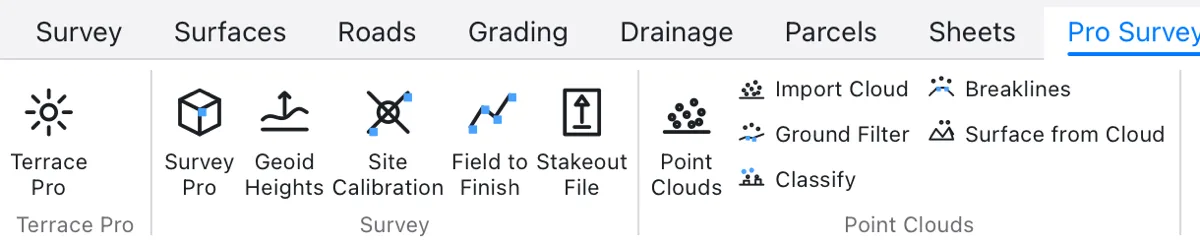
| Button | Command (aliases) | What it does |
|---|---|---|
| Survey Pro | SURVEYPRO (SPRO) | Opens the Survey Pro window: Geoid, Calibration, Field-to-Finish and Stakeout pages |
| Geoid Heights | GEOID (GEOIDHEIGHT, GH) | Geoid height at a point; converts point heights |
| Site Calibration | CALIBRATE (SITECAL, LOCALIZE) | Fits the local grid to GNSS control points and moves GNSS points into it |
| Field to Finish | FIELDTOFINISH (FTF, LINEWORK) | Draws linework from point codes and keeps it as surface breaklines |
| Stakeout File | STAKEOUTFILE (STAKEFILE, SOF) | Writes points, or an alignment's stakeout points, for a data collector |
| Point Clouds | CLOUDS (POINTCLOUDS, PCWINDOW) | Opens the Point Clouds window |
| Import Cloud | CLOUDIMPORT (PCIMPORT) | Reads a LAS or LAZ file into a point cloud of the project |
| Ground Filter | CLOUDGROUND (PCGROUND, GROUNDFILTER) | Finds the ground points |
| Classify | CLOUDCLASSIFY (PCCLASSIFY) | Sorts the other points into vegetation, buildings and noise |
| Breaklines | CLOUDBREAKLINES (PCBREAKLINES, PCBL) | Traces tops and toes of slopes and edges of pavement |
| Surface from Cloud | CLOUDSURFACE (PCSURFACE) | Makes a TIN surface from the ground and the breaklines |
Five more point cloud commands have no button: CLOUDLIST, CLOUDDISPLAY, CLOUDRESET and CLOUDEXPORT, CLOUDDELETE (see Point clouds on the command line). Every tool that changes the project is one undo step.
The Survey Pro window
The four survey tools share one window, with a page each: Geoid, Calibration, Field-to-Finish and Stakeout. Click Survey Pro (or type SURVEYPRO); it opens on the Geoid page, and you switch pages with the buttons at its top right. Close closes it. The window sits over the plan, so you see the results drawn behind it.
The ribbon's other four Survey buttons run the same tools as commands, at the command line. Both ways do the same work and save the same data in the project; use whichever you like. Each section below shows the window page first, then the command.
Geoid heights
GNSS receivers give ellipsoidal heights (h): heights above the WGS 84 ellipsoid, a smooth mathematical shape. Plans need orthometric heights (H): heights above mean sea level, which follows the geoid, the level surface of the Earth's gravity. The difference is the geoid height N, and H = h − N. In the Philippines N is tens of metres — about 43 m in Manila and 45 m at Teresa, Rizal — so it can't be ignored.
Terrace Pro carries the EGM2008 geoid model for the whole country (4°N to 22°N, 116°E to 128°E), on its 2.5-minute grid. Its source and accuracy are given on the Geoid page itself:
- It's the US National Geospatial-Intelligence Agency's grid, as PROJ distributes it, and public domain. Terrace interpolates it bilinearly, as PROJ does.
- EGM2008 matches levelled benchmarks to about 10 cm where gravity data are dense. In the Philippines it differs from NAMRIA's benchmarks by a few decimetres, with a regional tilt — fine for mapping. For engineering levels, tie the job to local benchmarks with a site calibration: its vertical plane takes up the geoid's local offset and tilt.
Terrace places points on the globe through the project's coordinate system, so set it first (Coordinate systems; e.g. PRS92 zone 3, EPSG 3123, as in the sample project, or UTM 51N).
On the Geoid page
- Open Survey Pro. The Geoid page explains the model, then has the tools.
- To read the geoid height anywhere, type a Latitude and Longitude in decimal degrees (they start at Manila, 14.5995 and 120.9842) and click Geoid Height.
- To change the elevations of all the project's points, click All Points to Orthometric (h − N) or All Points to Ellipsoidal (H + N).
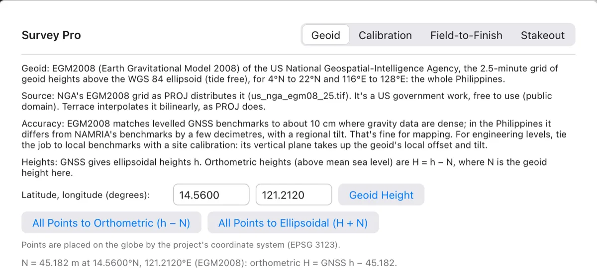
The conversion buttons change every point that has an elevation. Points that are locked, or outside the grid, are left alone. The change is one undo step (Geoid Heights).
Watch out Converting twice takes the geoid off twice. Convert once, right after you import GNSS points — or use the command, which lets you pick which points.
With the GEOID command
- Type
GEOID(GH) or click Pro Survey ▸ Geoid Heights. It asks Point for its geoid height or [Convert heights/Info]. - Click points in the plan: each one gets its geoid height in the log. Press Enter to finish.
- Or type C (Convert heights), choose Orthometric (the default; h − N) or Ellipsoidal (H + N), and type the point numbers, like 11-13,20 (Enter for all).
- Or type I (Info) to print what the geoid is, its source and its accuracy.

A conversion says how many points changed, shows the first one as an example (its N, and its height before and after), and lists the points skipped and why (no elevation, locked, outside the grid). Without a coordinate system, GEOID stops and asks you to set one.

Site calibration
A site calibration (also called a localization) fits your GNSS measurements to the job's local grid and benchmarks. You measure, with GNSS, a few control points whose local coordinates and elevations you know. Terrace finds the transformation that carries the measured coordinates onto the local ones, shows how well each point fits, and moves other GNSS points into the local grid with it.
Both sets of points must be in the project as points: the local ones (e.g. points 1–3, typed or imported from the control list) and the GNSS ones (e.g. 11–13, imported from the receiver). A pair is one local point and the GNSS point measured on it.
The models
- Horizontal fit: Rigid (rotation and shift: 3 parameters), Helmert (rotation, one scale and shift: a 2D similarity, 4 parameters; the default) or Affine (two scales and a skew too: 6 parameters, needs three or more points). They are fitted by least squares (Ghilani, Adjustment Computations, ch. 18).
- Vertical fit: None (heights as converted), Shift (one constant) or Plane (a shift and a tilt north and east, needs three or more points; the default).
- GNSS heights: take off the geoid (on by default): the measured heights are ellipsoidal, and EGM2008's N is taken off before the vertical fit, so the fit only has to take up the geoid's local error.
With too few points, Terrace falls back to a simpler model and says so: one point gives a shift only; two points can't make an affine fit or a plane. Points almost on one line fall back too.
On the Calibration page
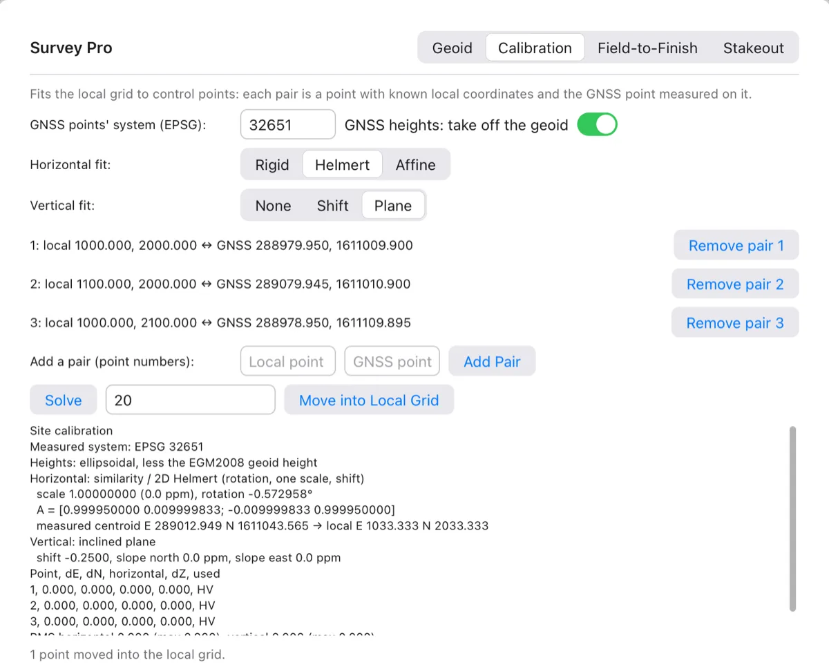
- Open Survey Pro and click Calibration.
- Check GNSS points' system (EPSG): the coordinate system the GNSS points' coordinates are in. It starts at the project's system; type 4326 if the GNSS points hold latitude and longitude.
- Choose the Horizontal fit and Vertical fit, and whether to take off the geoid.
- Under Add a pair (point numbers), type the Local point and the GNSS point and click Add Pair. Repeat for each control point. Each pair is listed with both coordinates and a Remove pair button. (Adding a pair for a local point that already has one replaces it.)
- Click Solve. The report appears under the buttons.
- Type the GNSS points to move in the box beside Solve (e.g. 20 or 1001-1020) and click Move into Local Grid.
Reading the report
- Horizontal: the model used, the scale (and its difference from 1 in ppm), the rotation, the 2×2 matrix A, and the centroids of the measured and local points.
- Vertical: the shift and the plane's slope north and east, in ppm.
- The residual table: for each pair, dE, dN, the horizontal residual, dZ, and whether it was used horizontally (H) and vertically (V). A residual is local minus transformed measured.
- The RMS and largest residuals, then notes in plain words.
The notes call out horizontal residuals over 0.03 and vertical residuals over 0.05 (project units) and say which point to check; a scale far from 1 (wrong system, feet vs metres, or a mismatched pair); a plane that tilts more than the geoid usually does; and a fit with no spare points, whose residuals are zero and prove nothing. When everything fits, the last line reads All residuals are within the tolerances. (The test survey above was made exactly, so its residuals are 0.000; real control shows millimetres to centimetres.)
Moving points reads each one's easting, northing and elevation as GNSS values (h) and replaces them with local ones. Locked points are left as they are. The calibration is saved with the project, so you can move more GNSS points into the grid later.
With the CALIBRATE command
CALIBRATE (SITECAL, LOCALIZE) shows a menu, Calibration (3 pairs) [Add/Remove/Model/SYstem/SOlve/REport/APply/Clear], and comes back to it after each choice. Enter picks SOlve when there are two pairs or more, Add before that.
| Option | What it asks and does |
|---|---|
| A Add | Point number with the local (known) coordinates, then Point number of the GNSS (measured) point there. |
| R Remove | The pair's name (the local point's number). |
| M Model | Horizontal fit [Rigid/Helmert/Affine], Vertical fit [None/Shift/Plane], then whether the measured heights are ellipsoidal and the geoid comes off [Yes/No]. |
| SY System | The GNSS points' EPSG code (4326 = WGS 84 latitude/longitude). Terrace refuses codes it doesn't know. |
| SO Solve | Fits the calibration and prints the report in the log. |
| RE Report | Prints the report again. |
| AP Apply | The GNSS points to move into the local grid (numbers like 1001-1020; you must type them). Ends the command. |
| C Clear | Removes all pairs and results. |
Field-to-finish linework
Field-to-finish draws the survey's lines — edges of pavement, centrelines, curbs, tops and toes of slopes, ditches, fences, buildings — from the codes the field crew typed on each point. You don't connect the dots by hand, and the lines follow the points: move a point or change its code and the line is redrawn. Lines that are breaklines can go straight into a surface.
How points are coded
Terrace reads the first word of each point's description as its code. A point makes lines when:
- its code matches a line code in the Field-to-Finish table (wildcards
*and?;EP*takes EP1, EP2… as separate lines), or - a description key with a Figure matches it (that key's layer and breakline setting are used).
Points are taken in point-number order. All points with the same code join into one line, until a line code letter after the code says otherwise:
| Letter (default) | Example | Meaning |
|---|---|---|
| B begin | EP1 B | Starts a new line with this point |
| E end | EP1 E | Ends the line at this point |
| C close | BLDG C | Ends the line and closes it back to its first point |
| A arc | CURB A | An arc starts here and passes through the next two points of the line |
| SC / EC | BANK SC … BANK EC | Start and end a smooth curve through the points between |
The built-in line codes are common Philippine and US topographic codes:
| Code | What | Layer | Breakline |
|---|---|---|---|
EP* | Edge of pavement | V-TOPO-PAVE | yes |
CL* | Road centreline | V-TOPO-PAVE | yes |
SH* | Edge of shoulder | V-TOPO-PAVE | yes |
CURB* | Curb (top back) | V-TOPO-CURB | yes |
GUT* | Gutter flow line | V-TOPO-CURB | yes |
TOP* | Top of slope | V-TOPO-SLOP | yes |
TOE* | Toe of slope | V-TOPO-SLOP | yes |
DIT* | Ditch / canal bottom | V-TOPO-DTCH | yes |
BANK* | Riverbank / creek bank | V-TOPO-WATR | yes |
FENCE* | Fence | V-TOPO-FENC | no |
WALL* | Wall | V-TOPO-WALL | no |
BLDG* | Building outline | V-TOPO-BLDG | no |
PL* | Property line | V-PROP-LINE | no |
On the Field-to-Finish page
- Open Survey Pro and click Field-to-Finish.
- If your crew uses other letters, change the Line code letters: begin, end, close, arc, curve start, curve end.
- Change the code table if needed. To add a code, type it in New code, set its Layer (V-TOPO-FIGR at first) and Breakline, and click Add Code; adding a code that's already there replaces it. Remove beside a code deletes it.
- Click Build Linework. The status beside it says how many lines there are, kept up to date.
- To put the breaklines in a surface, choose it under Breaklines into surface and click Keep Breaklines.
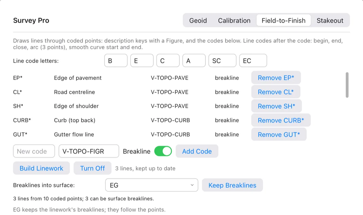
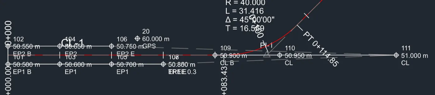
The notes under the page tell you what to fix: codes with only one point (no line), arcs that ended before their third point (drawn straight), smooth curves never ended, and breakline codes on points without elevations (drawn, but not used in surfaces).
The lines are named after their code, like EP1-1, and drawn on their codes' layers. In each surface you keep them in, they're breaklines named FTF …; the surface is rebuilt whenever the linework changes. Turn Off removes the linework and takes its breaklines out of the surfaces again.
With the FIELDTOFINISH command
- Type
FIELDTOFINISH(FTF) or click Pro Survey ▸ Field to Finish. The linework is built at once and the notes go to the log. (If no point has a line code, it says how to add some.) - If the project has surfaces, it asks Surface to keep the breaklines in or [None/Off]. Click or type a surface to keep the breaklines in it, press Enter (None) to leave surfaces alone, or O to turn the linework off.
The command uses the line code table and letters from the Field-to-Finish page; it doesn't change them.
Stakeout files
To set out a design, the field crew needs the points in their data collector. Stakeout File writes survey points, or stakeout points along an alignment, in the collector's own format.
| File kind | Extension | Notes |
|---|---|---|
| CSV point file (P,N,E,Z,D) | .csv | Point, northing, easting, elevation, description. Reads into almost anything. |
| Carlson SurvCE RW5 (stored points) | .rw5 | For an alignment with a design profile, the profile is also written as a SurvCE .pro file beside it. |
| Leica GSI-16 | .gsi | 16-digit words. |
| Leica GSI-8 | .gsi | 8-digit words: only for small coordinates; Terrace says so when they don't fit. |
| Sokkia SDR33 | .sdr | |
| LandXML 1.2 (points and alignments) | .xml | For an alignment, the alignment itself and its profiles go in too. |
For an alignment, Terrace makes points every interval and at the geometry points (BOA, PC, PT, EOA…), at each offset (− left, + right of the centreline). They're numbered from 1001. The description says the side, the offset and the station, like L5.00 0+020.00 or CL BOA 0+000.00. Centreline points get their elevation from the alignment's design profile; offset points have none. (For the station, offset and elevation table on screen or in a PDF, use the Free stakeout report.)
On the Stakeout page
- Open Survey Pro and click Stakeout.
- Choose Stake out: Points or Alignment.
- For points, type their numbers (like 1-20,25), or leave the box blank for all. For an alignment, choose it, and type the Interval (20 at first) and the Offsets (−5, 0, 5 at first).
- Choose the File kind, click Write File…, and choose where to save it.
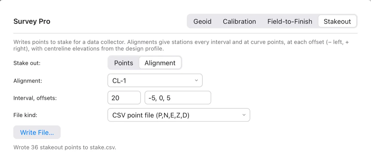
The start of that CSV file:
1001,2048.5000,1000.0000,,L5.00 BOA 0+000.00
1002,2043.5000,1000.0000,50.5000,CL BOA 0+000.00
1003,2038.5000,1000.0000,,R5.00 BOA 0+000.00
1004,2048.5000,1020.0000,,L5.00 0+020.00
1005,2043.5000,1020.0000,50.7000,CL 0+020.00
With the STAKEOUTFILE command
- Type
STAKEOUTFILE(SOF) or click Pro Survey ▸ Stakeout File. Answer Stake out [Alignment/Points] (Alignment when the project has one). - For an alignment: pick it, then Interval (0 = geometry points only) and Offsets (− left, + right), like -5,0,5. For points: Points (numbers like 1-20,25), Enter for all.
- Choose the File kind [CSV/RW5/GSI-16/GSI-8/SDR/LandXML] and type the file's path.
The command remembers the interval, offsets and file kind for next time.

Note Carlson's RD5 road file isn't a published format, so Terrace doesn't write it. For a road in SurvCE, send the alignment as LandXML and the profile as the .pro file.
Point clouds
Terrace Free can already make a surface from a LAS or LAZ file whose ground points are classified (see Point clouds (LAS and LAZ)). Many clouds aren't: a drone survey or a raw LiDAR file comes with every point "unclassified". Terrace Pro keeps the cloud in the project and works on it, in four steps:
- Ground: find the bare-ground points.
- Classify: sort the rest into vegetation, buildings and noise, by height above the ground.
- Breaklines: trace tops and toes of slopes and edges of pavement.
- Surface: a TIN from the ground with the breaklines, ready for contours, profiles and volumes.
Classes are the standard ASPRS LAS codes: 1 unclassified, 2 ground, 3/4/5 low/medium/high vegetation, 6 building, 7 low point (noise), 9 water, 11 road surface, 17 bridge deck, 18 high noise. The points are drawn in the plan coloured by class, on layers named PRO-CLOUD-GROUND, PRO-CLOUD-HIGH-VEG and so on; at most 20,000 points per cloud are drawn, picked evenly, so the plan stays quick. The cloud itself is saved inside the .terrace file.
The default lengths below are in metres; in a US-feet project they're scaled to feet.
The Point Clouds window
- Click Pro Survey ▸ Point Clouds (or type
CLOUDS). In a project with no cloud yet, the window offers Import LAS/LAZ…. - Click it and choose a
.lasor.lazfile. Every point is read.
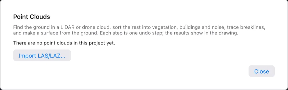
With a cloud in the project, the top of the window has:
- Cloud: which cloud the steps work on, if there are several.
- Import…: another cloud. Export LAS…: writes the cloud with its classes as a LAS file, for other programs.
- On the row below: Hide Points / Show Points: hides the points in the plan (the cloud stays). Reset Classes: back to the classes in the file. Delete: removes the cloud and its breaklines (surfaces made from it stay).
- How many points it has, and how many are in each class.
Under them are the four step tabs: Ground, Classify, Breaklines and Surface. Each step's settings are saved with the project, and what the step found is written in plain words at the bottom of the window.
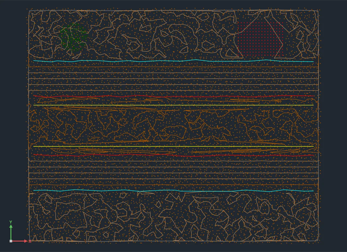
The example here is a small test scene of 8,300 points, 50 m by 40 m: a road on an embankment with side slopes, a few trees and a building on rolling ground.
Step 1: find the ground
Choose one of two well-known filters on the Ground tab and click Find the Ground. Ground points get class 2.
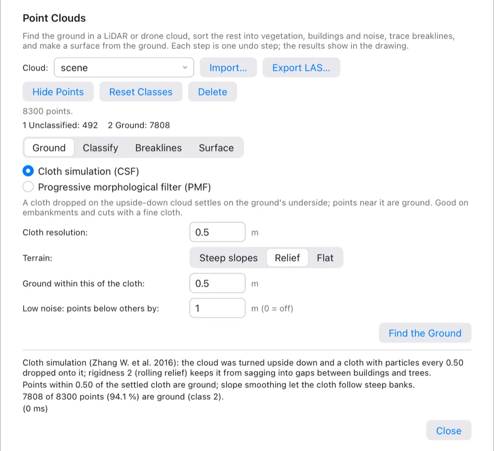
Cloth simulation (CSF), the default, turns the cloud upside down and drops a virtual cloth onto it; the cloth settles on the underside of the ground, and points near it are ground (Zhang W. et al., 2016). It does well on embankments and cuts.
- Cloth resolution: the spacing of the cloth's particles (0.5 m). Finer follows the ground more closely.
- Terrain: Steep slopes, Relief (the default) or Flat: how stiff the cloth is. A stiffer cloth doesn't sag into gaps between buildings and trees.
- Ground within this of the cloth: points at most this far from the settled cloth are ground (0.5 m).
Progressive morphological filter (PMF) takes the lowest point in each cell as a first ground model, then opens it with windows that grow; points that stand above it by more than a threshold are objects (Zhang K. et al., 2003). The defaults are PDAL's.
- Cell size (1 m).
- Widest object to remove: the largest window (33 m). Objects wider than this — a large building — stay as ground.
- Terrain slope (rise/run) (1): how fast the ground may rise; it raises the threshold with the window size.
- Initial height threshold (0.15 m) and Largest height threshold (2.5 m).
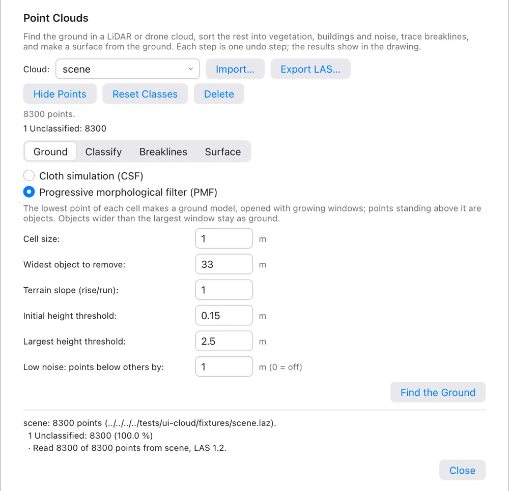
Both filters share Low noise: points below others by (1 m; 0 turns it off): points that lie this far below their neighbours, like reflections, become low noise (class 7) before the filter runs, so they don't drag the ground down.
Step 2: classify the rest
The Classify tab sorts the points that aren't ground by their height above it (a TIN of the ground points), their intensity, and — for buildings — whether they lie on flat or evenly sloping patches, like roofs. Run the ground filter first.
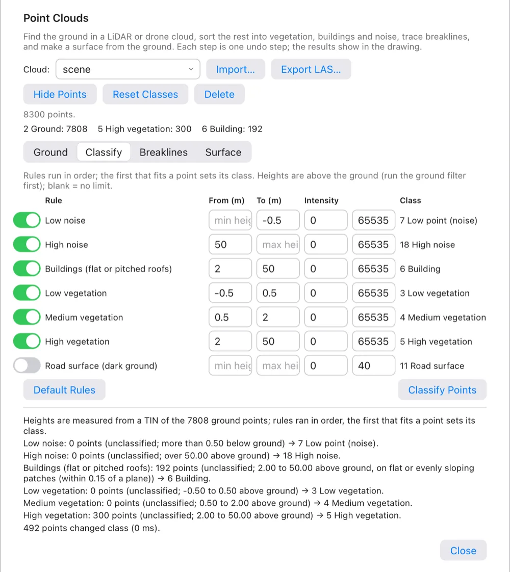
The rules run in order; the first rule that fits a point sets its class. Each rule has a switch, a height range above the ground (From, To; blank = no limit), an intensity range, and the class it gives:
| Rule | Height above ground | Class |
|---|---|---|
| Low noise | below −0.5 m | 7 Low point (noise) |
| High noise | above 50 m | 18 High noise |
| Buildings (flat or pitched roofs) | 2 to 50 m, on a plane within 0.15 m | 6 Building |
| Low vegetation | −0.5 to 0.5 m | 3 Low vegetation |
| Medium vegetation | 0.5 to 2 m | 4 Medium vegetation |
| High vegetation | 2 to 50 m | 5 High vegetation |
| Road surface (dark ground) — off | any; intensity 0 to 40 | 11 Road surface |
Change the numbers or the switches, then click Classify Points. The rules are saved with the project. Default Rules puts the table above back.
Step 3: breaklines
Breaklines keep a surface's triangles from cutting across sharp changes in the ground. On the Breaklines tab, Terrace traces them on a grid made from the ground points:
- Tops and toes of slopes (on): the edges of ground steeper than the limit. The line follows the strongest bend of the ground at each slope's edge.
- Edges of pavement (off at first): the edges of smooth, level ground whose intensity is in a range (pavement reads darker than grass and soil).
| Setting | Default | Meaning |
|---|---|---|
| Grid cell | 0.5 m | The grid the lines are traced on |
| Slopes are steeper than | 20 % | Steeper ground is slope; flatter is level |
| Smallest slope area | 20 m² | Smaller slopes are ignored |
| Shortest line | 5 m | Shorter lines are dropped |
| Simplify within | 0.1 m | Lines are simplified within this distance |
| Pavement intensity from / up to | 0 / 40 | Intensity range of pavement |
| Pavement roughness at most | 0.05 m | How far pavement may stray from a plane |
Click Find Breaklines. The result says what was found and, for pavement, what intensities the ground has (10 % below…, half below…), which helps you set the range for your scanner.
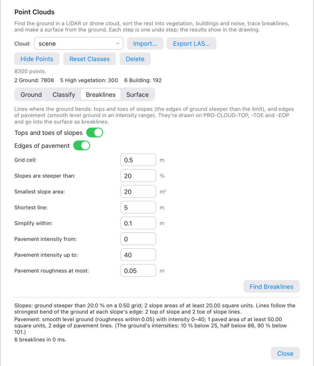
The lines are drawn on PRO-CLOUD-TOP (red), PRO-CLOUD-TOE (cyan) and PRO-CLOUD-EOP (yellow). Running the step again replaces the cloud's lines.
Step 4: the surface
On the Surface tab:
- Surface name: blank gives the cloud's name and "ground", like scene ground.
- Thin to one point per cell of (1 m; 0 = all points) and Point kept per cell: Average (the default) or Lowest.
- Use the breaklines (on): the cloud's breaklines become the surface's breaklines.
- Longest edge along the outside (10 m; 0 keeps all): long thin triangles around the edge are removed, so the surface doesn't bridge gaps in the ground.
Click Make Surface. It uses the ground, water and road surface classes (2, 9 and 11). Thinned points that lie right beside a breakline are left out, so the triangles follow the line.
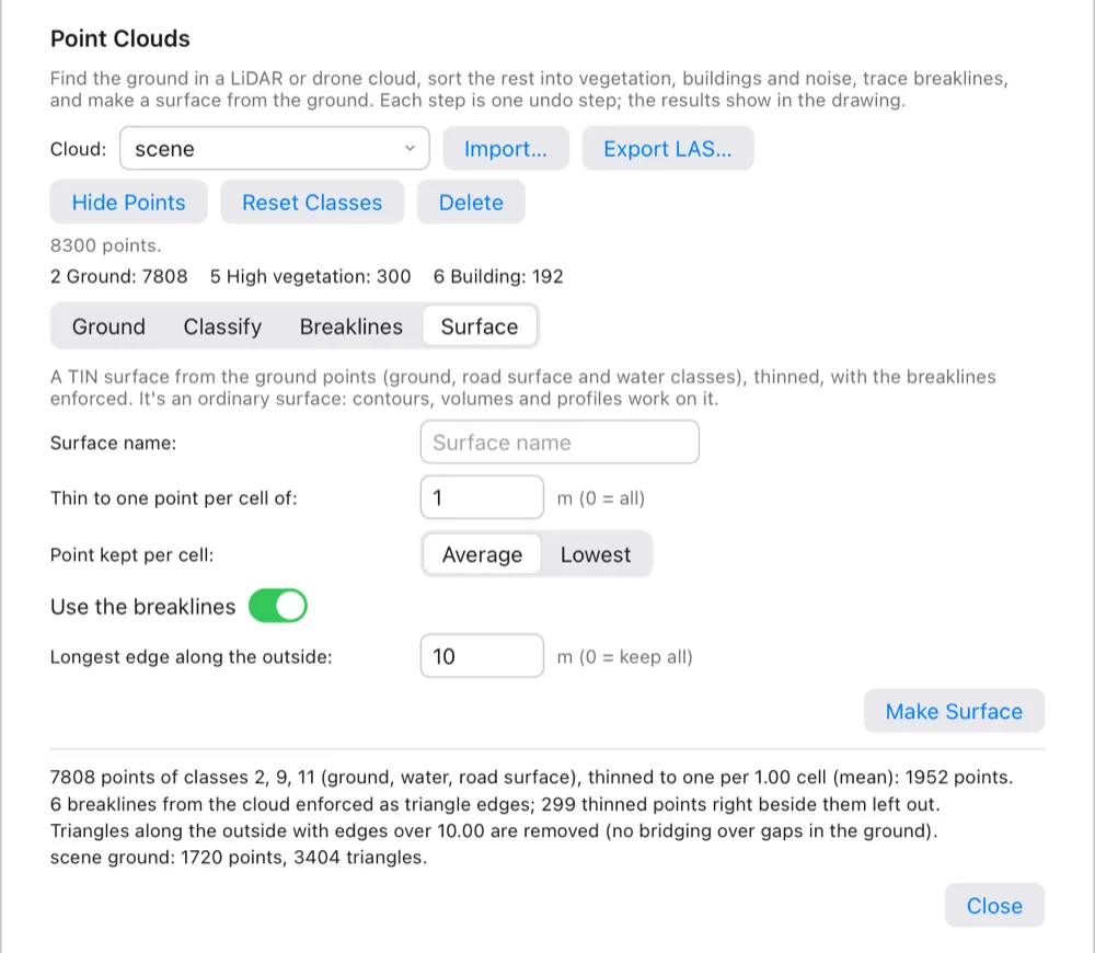
The result is an ordinary surface in the Project browser: contours, volumes, profiles and corridors work on it (see Surfaces).
Point clouds on the command line
Each step is also a command. With one cloud in the project, the commands use it; with several, they ask for the cloud's name first. Settings they don't ask for come from the window's tabs.
| Command | What it asks |
|---|---|
CLOUDIMPORT (PCIMPORT) | Point cloud file (.las, .laz), then Keep every n-th point (1 = all). The window's import keeps all points. |
CLOUDGROUND (PCGROUND, GROUNDFILTER) | Ground filter [Cloth/Morphological]. Cloth: Terrain [Steep/Relief/Flat]. Morphological: Widest object to remove, then Height above the ground model still taken as ground (the initial threshold). |
CLOUDCLASSIFY (PCCLASSIFY) | Nothing: runs the project's rules. |
CLOUDBREAKLINES (PCBREAKLINES, PCBL) | Find [Slopes/Pavement/Both], then Slopes are steeper than (%) and/or Pavement intensity up to. |
CLOUDSURFACE (PCSURFACE) | Surface name (the cloud's name and "ground"). |
CLOUDLIST (PCLIST) | Nothing: lists the classes and what was done to the cloud. |
CLOUDDISPLAY (PCDISPLAY) | Points [Show/Hide]. |
CLOUDRESET (PCRESET) | Nothing: the classes as in the file again. |
CLOUDEXPORT (PCEXPORT) | LAS file to write; the classes are written as they are now. |
CLOUDDELETE (PCDELETE) | Nothing: removes the cloud and its breaklines; surfaces made from it stay. |

CLOUDLIST: the cloud's history.How Terrace checks these tools
- Geoid: heights from Terrace's grid agree with PROJ's EGM2008 within 1 mm at over 400 places across the Philippines, directly and through UTM 51N and PRS92 zones.
- Site calibration: rigid, Helmert, affine and the vertical plane are checked against an independent least-squares solution (numpy, on Ghilani's observation equations) with noisy test control.
- Field-to-finish: linework is checked against Terrace's own figure builder and by hand for begin, end, close, arcs and curves.
- Stakeout files: CSV, RW5 and GSI files are read back with Terrace's own point and raw-data readers.
- Ground filters: on PDAL's Autzen test cloud (110,000 points), the PMF agrees with an independent implementation on over 99.99 % of points, and the cloth simulation with the CSF library on over 98.5 %. A synthetic scene with known ground, trees, a building, an embankment and a road checks the classes and the tops, toes and pavement edges.
Known limits: EGM2008 is a global model, so tie levels to local benchmarks with a site calibration; Carlson's RD5 road file isn't written; offset stakeout points carry no elevation.