
Pro: hydraulics and water networks
This chapter covers the Pro Analysis tab: culverts, ditches, detention ponds, flood maps, dam-break estimates and reservoir area–capacity tables, and the full analysis of water networks, the way EPANET does it. You'll be able to size a cross drain, check a lined ditch, route a storm through a pond, map what floods, and run a water main through a whole day with its reservoir, tank, demands, pumps and valves.
The Pro Analysis tab
Everything in this chapter needs Terrace Pro. In Terrace Free the buttons show a 🔒, and the commands open the Terrace Pro window instead of running.
The tab has two groups:
- Hydraulics: Hydro (the Hydro window), Culvert, Ditch, Detention Pond, Flood Map, Dam Break and Area–Capacity.
- Water Network: Water Analysis (the Water Network Analysis window), Run Analysis, Demand, Reservoir, Tank, Pump, Valve, Results Hour, Import EPANET and Export EPANET.

Each button runs a command you can also type; the command reference lists them all with their aliases. The commands ask at the command line with a default for every value, and remember your last answers. The Hydro window and the Water Network Analysis window show and edit everything in full. Every change is one undo step, and the results update when what they depend on changes (a surface, an alignment, a catchment).
Values are in the project's units: metres, m³/s and L/s in a metric project; feet, ft³/s and gpm in a US one.
Culverts
A culvert carries a creek or a ditch under the road. You check one to see how high the water stands at its inlet (the headwater) when the design flood passes. If the headwater is too high, the road floods or the water backs up onto land upstream.
Terrace follows FHWA HDS-5 (Hydraulic Design of Highway Culverts, 3rd ed., 2012). It works out the headwater two ways and takes the higher one:
- Inlet control: the entrance limits the flow, like a funnel. Terrace uses the regression equations behind the HDS-5 nomographs (Appendix A), for an unsubmerged inlet, a submerged one, and the transition between them.
- Outlet control: the barrel and the tailwater limit the flow. Terrace adds the entrance, friction and exit losses of the barrel flowing full to the outlet water level, taken as the tailwater or (critical depth + barrel height)/2, whichever is higher.
Making a culvert
This example adds a culvert where the creek crosses the Teresa Bypass in the sample project (Help ▸ Open the Sample Project).
- Click Pro Analysis ▸ Culvert, or type
CULVERT(CUL). - Click the inlet end of the barrel, then the outlet end. Terrace draws the culvert there and takes its length from the two points. Press Enter at the first prompt (None) for a culvert that isn't drawn (its length is then 20 m).
- At Pipe diameter (m) or [Box], type the diameter (default 0.91 m), or B for a box culvert: then give its span (width) and rise (height), 1.5 m each by default.

CULVERT asks for the barrel after the two points. - Give the Number of barrels (1), the Design flow (1 m³/s by default), the Inlet invert elevation (Terrace proposes the ground at the inlet less the barrel and 0.6 m of cover), the Outlet invert elevation (it proposes a 1 % fall) and the Tailwater depth above the outlet invert (0).
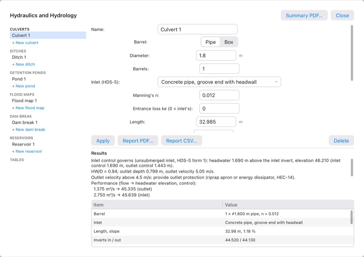
Terrace names it Culvert 1 and says the result. For a 1.8 m pipe carrying 5.5 m³/s with inverts 44.52 and 44.13:
- Inlet control governs (unsubmerged inlet, HDS-5 form 1): headwater 1.690 m above the inlet invert, elevation 46.210 (inlet control 1.690 m, outlet control 1.443 m).
- HW/D = 0.94; outlet depth 0.799 m, outlet velocity 5.05 m/s.
- Outlet velocity above 4.5 m/s: provide outlet protection (riprap apron or energy dissipator, HEC-14).
A new culvert gets Manning's n 0.012 and the inlet Concrete pipe, groove end with headwall (a box: Box, 30° to 75° wingwall flares). Change them in the Hydro window. On the plan, a drawn culvert is an outline of its barrels with a flow arrow and a label such as Culvert 1: 1-⌀1.80 m, HW 46.21, on layer C-HYDR-CULV.
The culvert's fields
| Field | What it is |
|---|---|
| Barrel | Pipe (circular) or Box. |
| Diameter, or Span (width) and Rise (height) | The barrel's size. |
| Barrels | How many barrels side by side; the flow is shared equally. |
| Inlet (HDS-5) | The inlet's shape and edge: eight pipe inlets (concrete square edge or groove end, corrugated metal headwall, mitered or projecting, beveled rings) and eight box inlets (wingwall flares, chamfers, bevels). Each has its HDS-5 coefficients in the Tables page. |
| Manning's n | Roughness of the barrel (0.012 for concrete). |
| Entrance loss ke (0 = inlet's) | 0 uses the inlet's own ke from HDS-5 Table C.2. |
| Length, Inlet invert, Outlet invert | The barrel's length and its ends; the slope follows from them. |
| Design flow, Tailwater depth | The flood to pass, and the water depth at the outlet. |
| Allowable HW (0 = none) | The highest headwater elevation you accept. Terrace says whether the headwater is above or below it. |
| Road crest (0 = none) | The road's lowest point over the culvert. Terrace warns The road overtops when the headwater is higher. |
| Inlet point x,y (drawn), Outlet point x,y | Where it's drawn; leave them empty for a culvert that isn't drawn. |
Terrace also warns when HW/D (headwater over barrel height) is above 1.5, when the barrel is flat or slopes backwards, and when the outlet velocity is above 4.5 m/s (15 ft/s). The table under the results lists the barrel, inlet, length and slope, inverts, flow, the inlet and outlet control headwaters, the controlling one, critical and normal depth, and the outlet depth and velocity.
The culvert's report also has a performance curve: the headwater at 25 %, 50 % … 200 % of the design flow, with the control at each. Its rows are at the end of the window's results (scroll down), and in Report PDF…, Report CSV… and HYDROREPORT.
Ditches and open channels
A roadside ditch has to carry its flow without spilling and without scouring its lining. Terrace finds the normal depth (the steady depth of uniform flow) by Manning's equation, then checks the freeboard, the velocity and the shear on the bottom against the lining.
- Click Pro Analysis ▸ Ditch, or type
DITCH(DIT). - Choose the Ditch shape: Trapezoidal (the default), Rectangular or V.
- Give the Bottom width (0.5 m; not for a V), the Side slopes as horizontal per 1 vertical (1.5, or 2 for a V; not for a rectangle), the Ditch depth (0.6 m) and the Longitudinal slope in % (0.5).
- At Design flow (m³/s) or [Catchment], type the flow (0.5 m³/s), or C and click a catchment: Terrace then takes the flow by the rational method from the catchment's area, C and time of concentration, and asks for the Return period (10 years). The rainfall comes from the project standard's first rainfall station.
- At Lining, press Enter for Concrete, unfinished, or type a name or part of one from the lining table, such as
class Cfor grass class C.
A 0.5 m trapezoidal ditch on a 2 % slope, lined with grass class C and carrying 0.25 m³/s, gives:

What Terrace checks:
- Capacity: whether the section can carry the flow at all at this slope.
- Flow regime: the Froude number, subcritical or supercritical. Between 0.86 and 1.13 it warns that near-critical flow makes a wavy, unstable surface.
- Freeboard: the ditch depth less the flow depth, against the freeboard required (0.15 m; 0.5 ft). If it's short, Terrace says how deep the ditch must be.
- Velocity: against the lining's permissible velocity (bare soils), and in metric projects a note when it's under 0.6 m/s, where silt may settle.
- Shear: the bottom shear τ = γyS (HEC-15) against the lining's permissible shear (grass, riprap, soils).
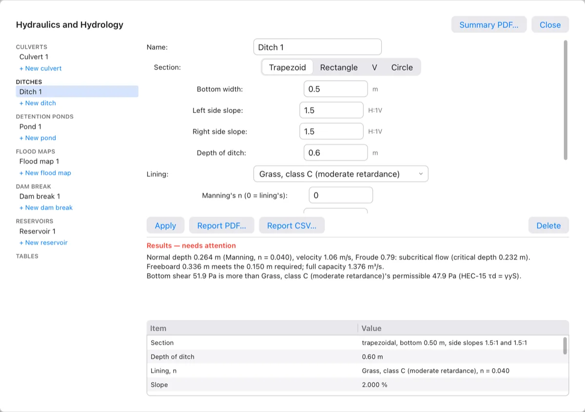
In the Hydro window a ditch can also be a Circle (a pipe flowing part full, by its Diameter), have different Left side slope and Right side slope, its own Manning's n (0 = lining's), a Freeboard required, and take its flow from a catchment (Flow from catchment, with Return period and Rainfall station (IDF)) or a typed Design flow. Ditches aren't drawn on the plan; they're checks of a typical section.
Detention ponds
A detention pond holds back storm runoff and lets it out slowly, so the peak flow downstream is lower. To check one you need three things: how much the pond holds at each level (the stage–storage curve), how much its outlets let out at each level (stage–discharge), and the storm coming in. Terrace routes the storm through the pond by the storage-indication (modified Puls) method (Chow, Maidment & Mays, Applied Hydrology, §8.2) and reports the peak in and out, the highest water level and the freeboard.
Making a pond
- Click Pro Analysis ▸ Detention Pond, or type
POND(DPOND). - Pick the pond's surface: its finished grading (see Grading).
- Click a point inside the pond. Only water connected to this point counts as the pond. Terrace follows the water downhill from the point: where it ends in a hollow, that low point is the pond's bottom. Where it runs off the edge of the surface (natural ground with no hollow), the bottom is the lowest ground at the point, where the pond's water first stands.
- Give the Top of the pond (Terrace proposes the surface's highest point) and the Low-flow orifice diameter (0.3 m).
- Click the catchment that drains to the pond, or type R (Rational) and give the Drainage area in ha (5), the Runoff coefficient C (0.6) and the Time of concentration in minutes (15). When the project has no catchments, Terrace asks for these straight away.

POND on the sample's creek, with the creek catchment as inflow.
Terrace gives the pond two outlets: the orifice at the bottom (the command line says its level), and a 3 m broad-crested emergency spillway 0.6 m below the top (0.3 m freeboard + 0.3 m). The inflow is the 25-year storm of the standard's first rainfall station by the modified rational method. It tries storm durations and keeps the one that fills the pond highest (the critical duration). Edit any of it in the Hydro window.
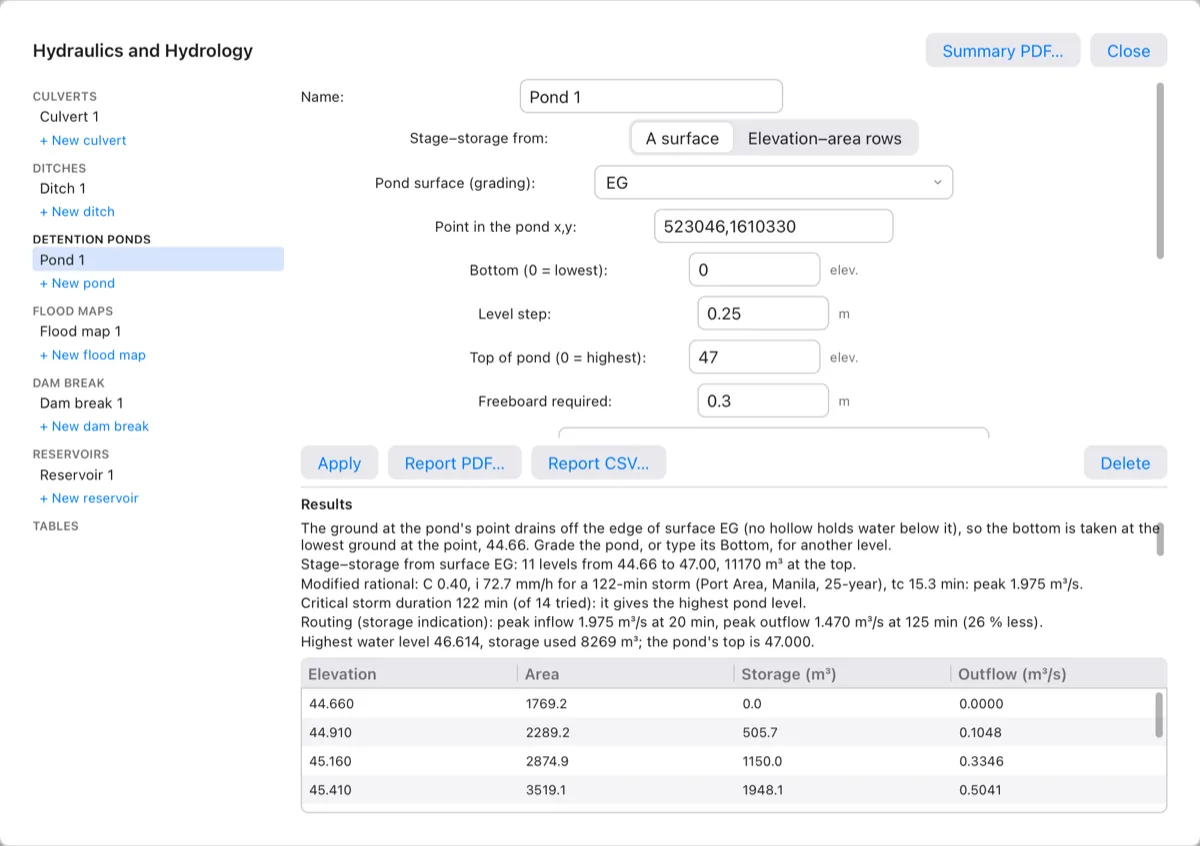
The pond's bottom On natural ground such as EG, the creek here runs on past the pond and off the surface, so no hollow holds water below the point: Terrace starts the table at the lowest ground at the point (44.66) and puts the orifice there, and the results say so. The storage counts from the bottom up, in the water connected to the point, which on EG includes the creek downstream. For a real pond, pick its grading. To use another level, type it in Bottom, move the orifice's invert in Outlets, then click Apply.
The pond's fields
| Field | What it is |
|---|---|
| Stage–storage from | A surface (water on the grading, exact per triangle) or Elevation–area rows: Elevation,area; … typed as 100,800; 101,1300; 102,1900 (m and m²). |
| Pond surface (grading), Point in the pond x,y | The surface, and a point in the water. |
| Bottom (0 = lowest), Level step | Where the table starts, and its step (0.25 m). |
| Top of pond (0 = highest), Freeboard required | The top of the embankment, and how far below it the water must stay (0.3 m). If the water goes over the top, Terrace says The pond overtops. |
| Outlets | One outlet per part, separated by ;: kind invert size, then any of w= (width), h= (height), c= (coefficient), n= (how many), r= (rating rows). Kinds: orifice (size = diameter, or w= and h= for a rectangle), weir (sharp-crested, length w=), broad (broad-crested, size = length), vnotch (size = angle in degrees), riser (size = pipe diameter, crest at the invert) and rating (r=46:0,47:1.5: level:flow pairs). Example: orifice 44.6 0.6; broad 46.4 3. Default coefficients: orifice 0.60, sharp weir 1.84, broad-crested 1.70, V-notch Cd 0.585. |
| Starting level (0 = lowest outlet) | The water level when the storm starts. |
| Inflow | Modified rational, SCS unit hydrograph or Table. |
| From catchment | A catchment of the project (its area, weighted C and time of concentration), or (none: the values below): Drainage area (ha for rational, km² for SCS), Runoff coefficient C or Curve number CN, and Time of concentration. |
| Rainfall station (IDF), Return period | The rainfall intensity–duration–frequency curve and the storm's return period (25 years). |
| Storm duration (0 = critical) | 0 searches for the duration that fills the pond highest. |
| Time (min),flow; … | For Table: the inflow hydrograph, typed. |
| Time step | The routing step (5 min). |
The SCS unit hydrograph follows NRCS NEH-630: the station's rainfall arranged as a design storm by alternating blocks, losses by the curve number, and the dimensionless curvilinear unit hydrograph (Table 16-1). The modified rational hydrograph is a triangle when the storm lasts as long as the time of concentration, and a trapezoid when it lasts longer.
On the plan a pond built from a surface shows its outline at the highest water level, labelled Pond 1: max WL 46.61, on layer C-HYDR-POND.
Flood maps
A flood map shows what's under water and how deep, for a flat water level (a lake, a pond, a design flood level) or for a water surface that slopes along a river. Terrace clips every triangle of the ground surface exactly at the water, sums the area and the volume, and draws the flooded area in three depth bands. The default bands follow the PAGASA/DPWH flood hazard levels: under 0.5 m low, 0.5–1.5 m medium, over 1.5 m high.
- Click Pro Analysis ▸ Flood Map, or type
FLOODMAP(FLOOD). - Pick the ground surface (here
EG). - At Water [Level/Profile], press Enter for a level.
- Give the Water level. Terrace proposes a quarter of the way up the surface's range of elevations.
- Click a point in the water, so that only water connected to it counts, or press Enter (All) for every low spot under the level.
For water at 46.50 in the sample's creek:

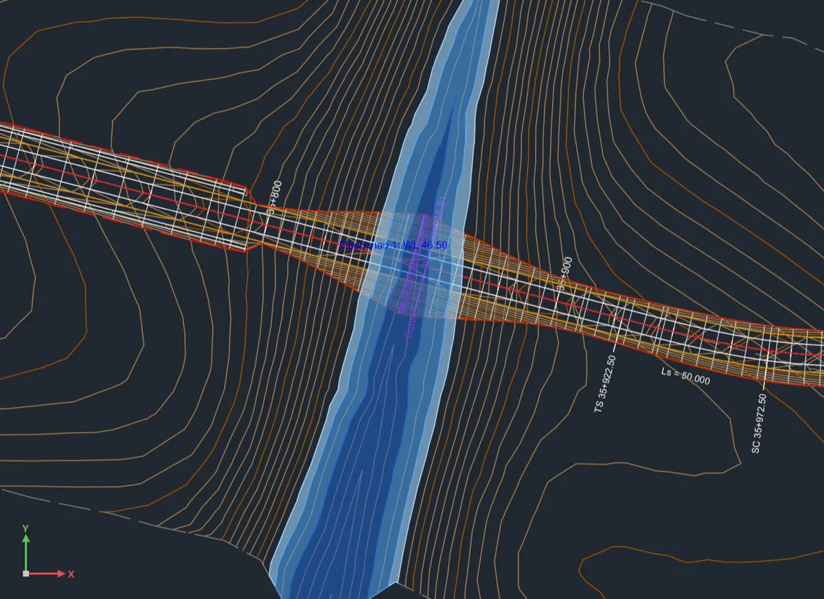
C-HYDR-FLOD. The bands cross the road because EG is the ground before the road was built.A water surface along a river
For a river, the water surface falls downstream. Get the water surface elevations at a few stations (from HEC-RAS, a high-water-mark survey, or a hand calculation), then:
- Start
FLOODMAP, pick the surface, and type P (Profile). - Pick the river's alignment (draw it along the river first, see Alignments).
- Type each station and its water elevation as
station,elevation, with the station as a plain number (120,45.6for 0+120). Press Enter when done; at least two are needed.
Each point of the ground takes the water surface at its station along the river, interpolated linearly. Points before the first station or after the last stay dry. In the Hydro window, Largest offset (0 = any) keeps the water within that distance of the river.
The flood map's fields
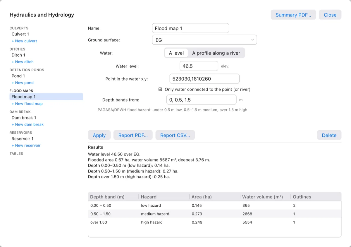
Only water connected to the point (or river) leaves out separate hollows. Depth bands from lists the lower limit of each band (0, 0.5, 1.5); type your own to change them. The table lists each band's area, water volume and number of outlines.
Dam break (a screening estimate)
A dam-break estimate tells you roughly how big the flood from a failed embankment dam would be and how far it reaches. Use it to screen a site or to decide whether a full study is needed. It is not a dam safety study: that needs an unsteady flow model such as HEC-RAS, and Terrace says so under every result.
How Terrace estimates it:
- The breach (the gap that opens in the dam) by Froehlich (2008): average width, side slopes and formation time from the reservoir volume and the breach height. Overtopping and piping failures use different factors.
- The outflow hydrograph: the breach grows over its formation time, water flows through it as over a broad-crested weir, and the reservoir drains. Terrace also gives Froehlich's 1995 peak-flow formula as a check.
- Downstream, if you give a river alignment: cross-sections cut from the surface every so often along the river, Muskingum–Cunge routing between them, and the peak flow, its arrival time and the peak water level (at normal depth) at each section, with the flooded area in depth bands.
- Click Pro Analysis ▸ Dam Break, or type
DAMBREAK(DBREAK). - Pick the Reservoir surface, and click a point in the reservoir.
- Give the Dam crest elevation, the Water level at failure (the crest by default) and the Breach bottom elevation (the surface's lowest point by default).
- Choose the Failure mode: Overtopping (the default) or Piping.
- Pick the River alignment downstream, or press Enter (None) for the breach outflow only. Terrace skips this step when the project has no alignments.
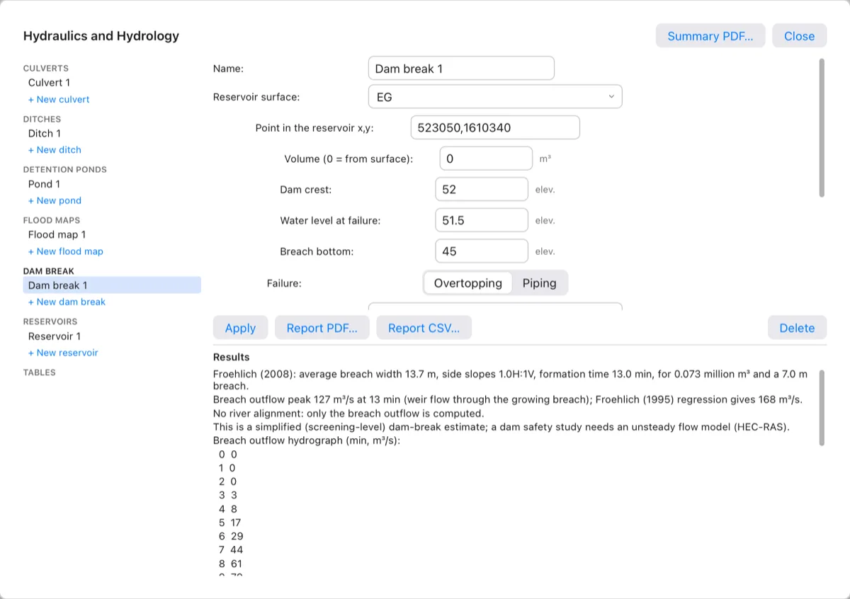
In the Hydro window you can also set:
- Reservoir surface: (none: a volume), with a typed Volume (0 = from surface) when you know the storage but have no surface. Terrace then treats the reservoir as vertical-walled.
- River downstream and River surface (the reservoir's by default).
- Manning's n of the valley (0.045), Section spacing (250 m), Section half width (400 m), Time step (60 s), and Depth bands from.
With a river, the table lists every section's station, distance, peak flow, peak time, peak stage, depth and top width, and the plan labels each section with its peak flow and water level, on layer C-HYDR-DAMB. The breach outflow hydrograph (time, flow) is at the end of the window's results, and in the report (PDF, CSV or HYDROREPORT).
Limits Breach parameters come from regressions on past failures, with wide scatter. Normal depth at each section ignores backwater and the flood's own dynamics. Use the numbers to compare and to screen, not to set evacuation lines.
Reservoir area–capacity
An area–capacity table gives a reservoir's water area and stored volume at each level. You use it in reservoir operation studies, to set the normal and dead storage levels, and to report live storage.
- Click Pro Analysis ▸ Area–Capacity, or type
AREACAPACITY(AREACAP,ACAP). - Pick the reservoir's surface. Click a point in the reservoir, or press Enter (All) to count every low area.
- Give the Elevation step (1 m) and the Normal water level (0 = none).
Terrace lists the table at the command line (up to 40 rows) and keeps it as Reservoir 1. Areas and volumes are exact on the surface's triangles. The plan outlines the water at the normal level (or the top level), labelled Reservoir 1: WL 47.00, on layer C-HYDR-RESV.
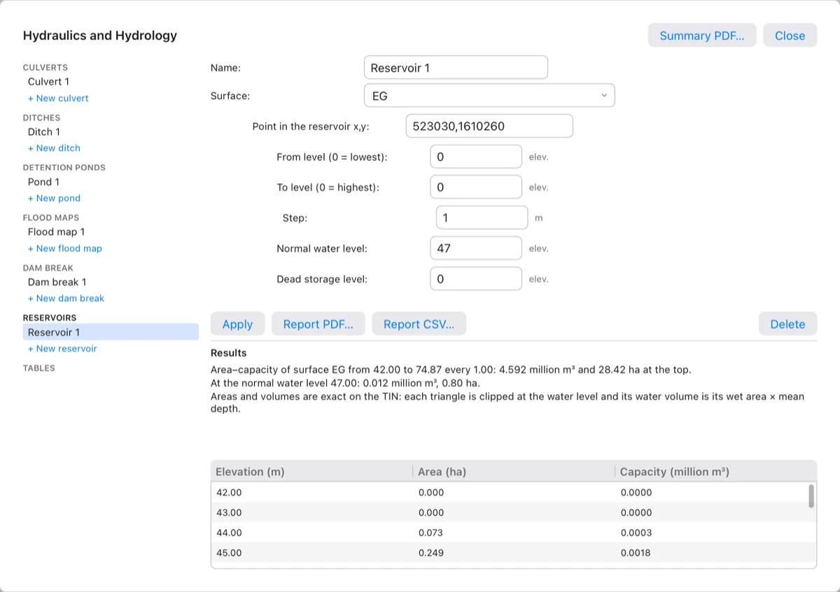
In the window you can also set From level (0 = lowest) and To level (0 = highest), and a Dead storage level. Terrace then reports the dead storage below it and the live (active) storage between it and the normal level. US projects get acres and acre-feet.
The Hydro window
Click Pro Analysis ▸ Hydro, or type HYDRO (HYD). The window, titled Hydraulics and Hydrology, lists every hydro object of the project on the left, by kind: Culverts, Ditches, Detention ponds, Flood maps, Dam break, Reservoirs and Tables.
- Click a name to edit it. The fields are at the top right; the results in words and the object's table are below them.
- + New culvert, + New ditch and so on make one with defaults from the project: its first surface, its first alignment as a dam-break river, the standard's first rainfall station. A new pond on a project without surfaces starts from elevation–area rows.
- Apply stores the fields as one undo step and recomputes. If a field isn't a number, Terrace says which one in red and keeps the object as it was.
- Report PDF… and Report CSV… save the selected object's report; Delete removes it.
- Summary PDF… (top right) saves one report of every hydro object with its result, and Close closes the window.
Points are typed as x,y, rows as a,b; c,d. A heading in red, Results — needs attention, means a check failed: a ditch that can't carry its flow or would erode, a culvert over its allowable headwater, an overtopped road or pond, short freeboard.
The Tables page
Click Tables in the list. The two tables are saved with the project, so each project can have its own values.
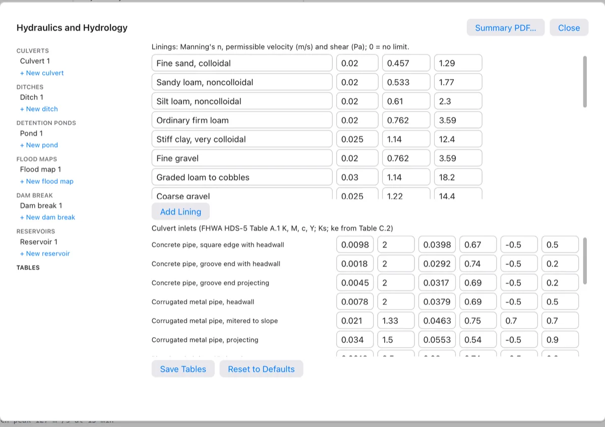
- Linings: name, Manning's n, permissible velocity and permissible shear (0 = no limit). Terrace ships 21 linings: bare soils from Fortier & Scobey (Chow Table 7-3), grass classes A–E and riprap of D50 150 and 300 mm (HEC-15), grouted riprap, stone masonry, and concrete (trowel finish, unfinished). Add Lining adds a row; clear a name to remove its row.
- Culvert inlets: for each inlet, the HDS-5 Table A.1 coefficients K, M, c and Y, the slope correction Ks, and the entrance loss ke (Table C.2).
Save Tables stores both tables (one undo step). Reset to Defaults brings back the published values.
Hydro reports and the list
HYDROREPORT(HYREP): type an object's name (the last one made is the default). Then press Enter to show the report at the command line, or type a path ending in.pdfor.csvto save it. PDFs carry your firm's name and logo (see Terrace Pro).HYDROLIST(HYLIST): one line per object with its main result, and — needs attention after any that failed a check.HYDRODELETE(HYDEL): deletes an object by name.

The reports: Culvert Hydraulics (with the performance curve), Ditch Hydraulics, the pond's stage–storage–discharge table with its routing, the flood map's depth bands, the area–capacity table, and the dam break's breach and downstream peaks with the outflow hydrograph. See also Reports.
How Terrace checks this
The hydro calculations are tested against published worked examples and an independent Python implementation of the same equations:
- Culverts: FHWA HDS-5 (2012) Design Guidelines DG 1.3 and DG 1.4.
- Normal depth: Chow (1959) Example 6.2.
- Pond routing: Chow, Maidment & Mays (1988) Example 8.2.1.
- The SCS unit hydrograph: NRCS NEH-630 ch. 16 Example 16-1 and TR-55 Example 2-1.
- Breach parameters: the Froehlich (2008) worked example in USACE HEC TD-39.
What it doesn't do: no gradually varied flow profiles in ditches or culvert barrels beyond the HDS-5 method, no unsteady river hydraulics (the dam break is a screening estimate), and no sediment.
Water network analysis
The Drainage tab lays out water mains as pressure networks (see Water mains). Terrace Pro analyses them the way EPANET 2.2 does: given where the water comes from and where it's used, it finds the flow in every pipe and the pressure at every fitting, hour by hour through a day.
- A reservoir is a source with a fixed water level: a spring box, an elevated source, or a connection to an existing main.
- A tank is storage whose level rises and falls through the run.
- A demand is the average water use at a fitting (L/s). A pattern multiplies it hour by hour, for example low at night and high in the morning.
- A pump or a valve takes the place of a pipe of the network.
- An extended-period run solves every hour (or step) of the duration, 24 hours by default, moving the tank levels between steps.
The analysis checks each junction's pressure against the network's Lowest pressure and Highest pressure (DPWH/LWUA practice: 7 to 70 m) and each pipe's velocity against Highest velocity (3 m/s). These are the pressure network's Properties.
Setting up a main
This example lays a main along the north side of the Teresa Bypass in the sample project. Its source is at the west end, and a tank floats on the system at the east end.
- Lay the main with Drainage ▸ Pressure Network (
PRESSURENETWORK), as in Water mains. Here it's named Teresa Water Main: 3 pipes (PVC 150 mm) W-1 to W-3, and fittings F-1 to F-4. - Click Pro Analysis ▸ Reservoir (
WNRESERVOIR,WNR). Click the fitting, or type its name (F-1). Give the Water level of the reservoir; Terrace proposes 30 m above the fitting.
F-1 becomes the source at 89.66 m. - Click Pro Analysis ▸ Demand (
WNDEMAND,WND). Pick a fitting and give its Average demand in L/s. At Demand pattern, press Enter for the network's default pattern, or typedailyfor a residential day: Terrace adds a 24-hour pattern with a morning and an evening peak that averages 1. Pick the next fitting, or press Enter to finish. Here F-2 uses 12 L/s and F-3 10 L/s, bothdaily.
A demand and its pattern. - Click Pro Analysis ▸ Tank (
WNTANK,WNT). Pick the fitting (F-4) and give the Bottom elevation (the fitting's elevation by default; here 85.5 m, an elevated tank), the Inside diameter (10 m), the Lowest and Highest water level above the bottom (0.5 and 5 m) and the Water level at the start (80 % of the highest). Terrace says the tank's working volume: 353 m³.
WNTANK asks for the tank's shape and levels.
The other elements:
- Pump (
WNPUMP,WNP): pick the pipe that is the pump; it pumps from the pipe's start to its end. Give its Design flow and Design head (10 L/s at 40 m by default). Terrace makes a one-point pump curve, which EPANET extends to 133 % of the head at no flow and no head at twice the flow. Or type P for a constant Pump power in kW. - Valve (
WNVALVE,WNV): pick the pipe that is the valve (flow from its start to its end), then its type and setting:Type What it does Setting (default) PRV, pressure reducing Keeps the pressure below it from rising above the setting. 30 m PSV, pressure sustaining Keeps the pressure above it from falling below the setting. 20 m PBV, pressure breaker Makes a fixed pressure drop. 10 m FCV, flow control Limits the flow. 10 L/s TCV, throttle control Adds a loss coefficient K. 5 WNCLEAR(no ribbon button; Clear… in the window's Setup tab): pick a fitting or a pipe to make it plain again (no demand, source, pump or valve).
Everywhere you can click the fitting or pipe on the plan, or type its name.
Running the analysis
Click Pro Analysis ▸ Run Analysis, or type WNRUN (WNA). With one network it runs at once; with several, pick a pipe of one, or press Enter (All). The command line sums up the run, and the plan shows the results.
Then click Water Analysis (WATERNET, WN) to open the Water Network Analysis window. It opens on the selected network, or the first one; with several networks, a menu at the top switches between them.
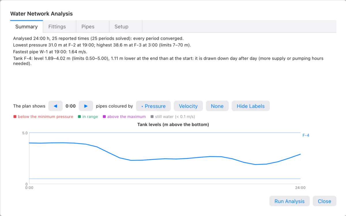
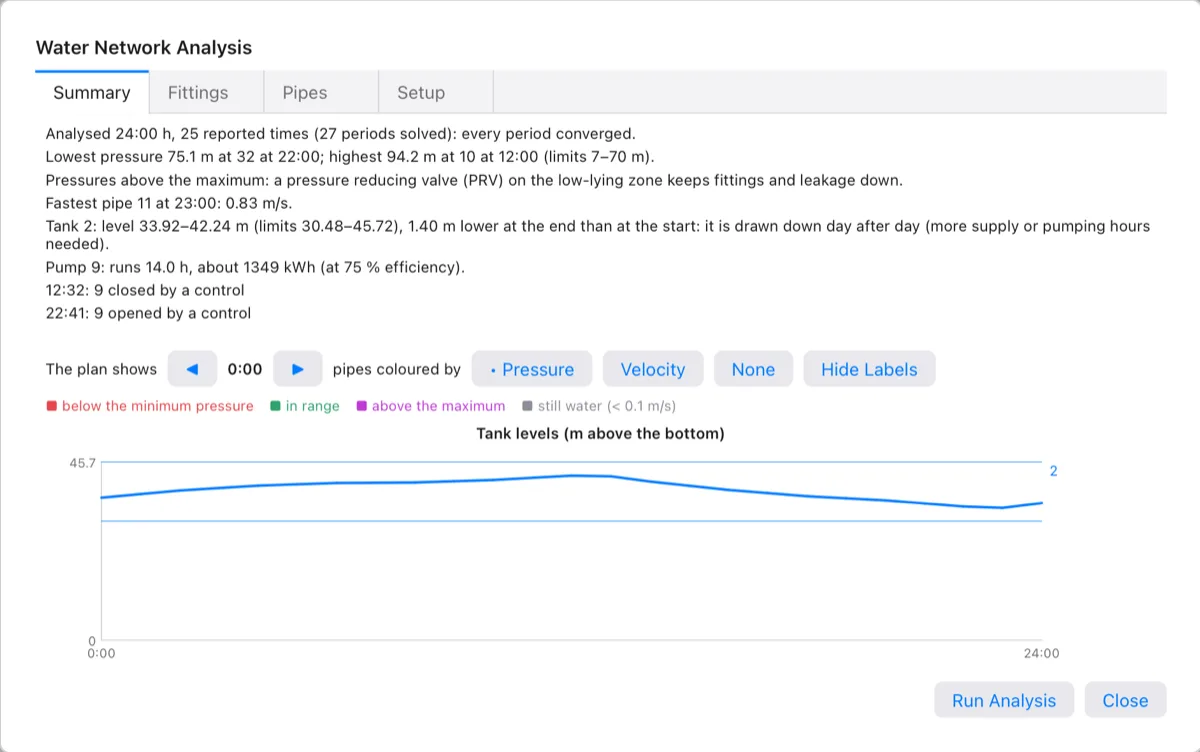
The Summary tab tells you, in plain words:
- whether every period converged;
- the lowest and highest pressure, where and when, against the limits, with advice when they're out of range (larger pipes, a higher source, a booster pump or a tank for low pressure; a PRV for high pressure);
- the fastest pipe;
- each tank's range of levels, and whether the day balances or the tank empties or fills;
- each pump's running hours and energy;
- what controls did and when.
Under it, The plan shows ◀ 0:00 ▶ steps through the reported times, the buttons colour the pipes by Pressure, Velocity or None, and Hide Labels / Show Labels turns the plan labels off and on. The chart shows each tank's level through the run, with its lowest and highest levels as thin lines.
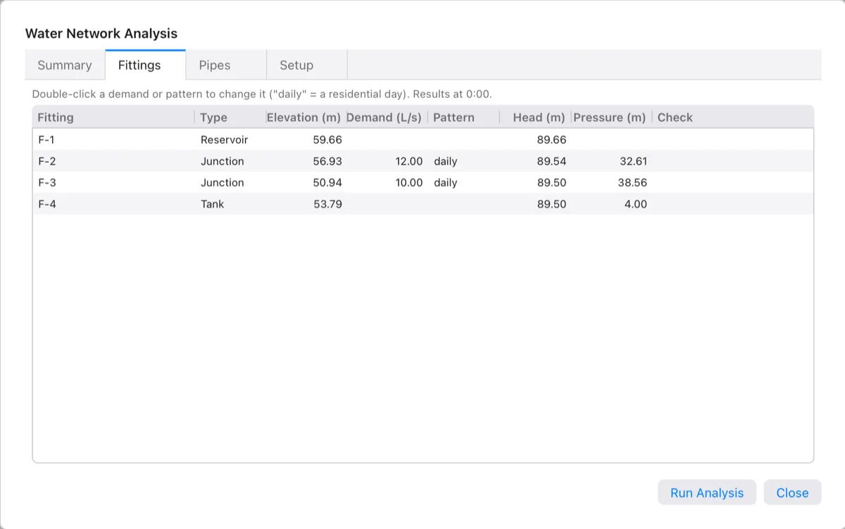
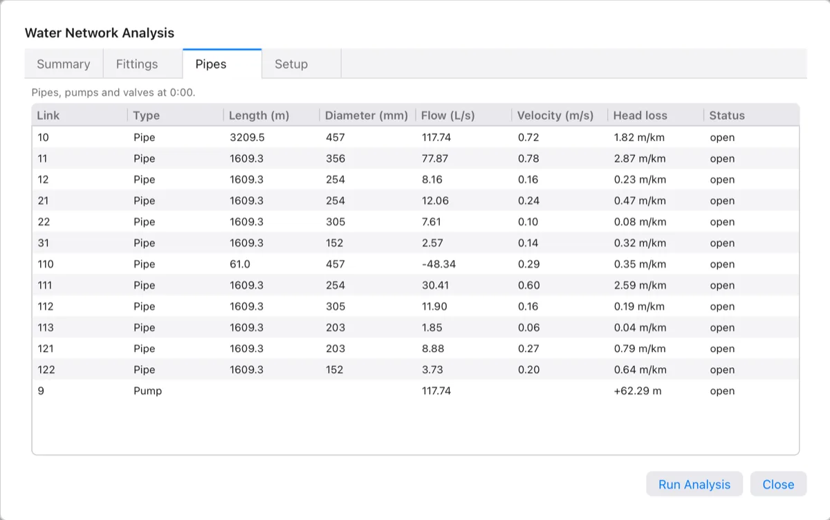
The Fittings tab lists every fitting with its type, elevation, demand, pattern, and the head, pressure and check at the hour shown. Double-click a Demand to change it (0 or empty removes it), or a Pattern to name another one. The Pipes tab lists every pipe, pump and valve with its length, diameter, flow, velocity, head loss (m/km for pipes; the head a pump adds) and status.
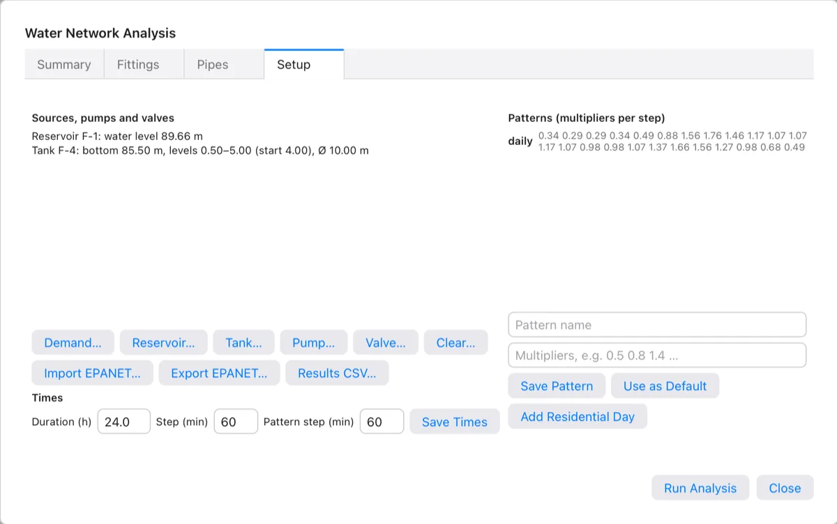
The Setup tab lists the sources, pumps and valves, and has buttons that close the window and start the matching command. Under Times:
- Duration (h): 24 by default; 0 runs a single steady period.
- Step (min): the hydraulic step, 60 by default.
- Pattern step (min): how long each multiplier of a pattern lasts, 60 by default.
Click Save Times, then run again. Under Patterns, type a Pattern name and its Multipliers (one per pattern step, separated by spaces), then click Save Pattern. Use as Default makes the named pattern apply to every demand that names none. Add Residential Day adds the daily pattern.
When you change the network or its setup after a run, the Summary says The network or its setup changed since this analysis: run it again, and the tables wait for a new run. Run Analysis at the bottom of the window runs it.
Results on the plan
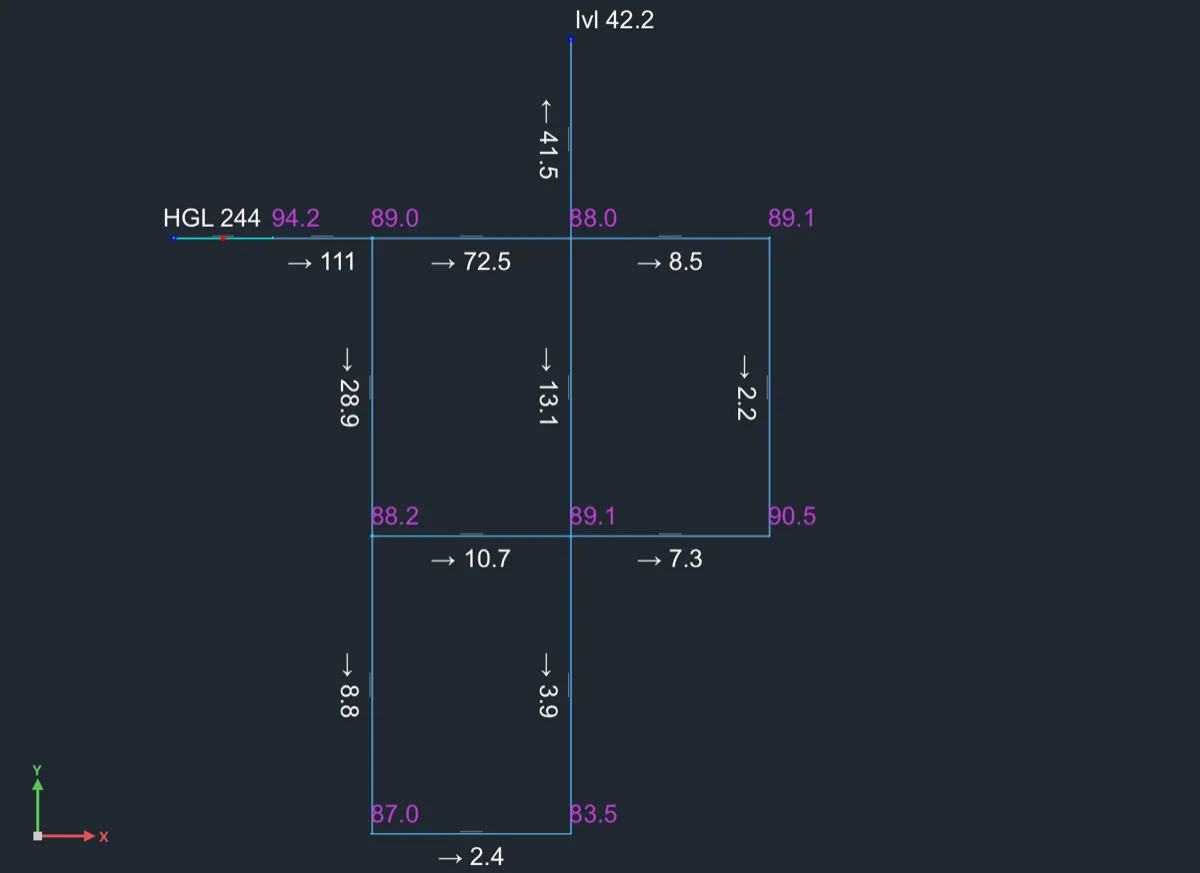
Click Pro Analysis ▸ Results Hour (WNTIME). Give the Hour to show and how to Colour pipes by: Pressure, Velocity or None. Pipes are red below the minimum pressure, green in range, purple above the maximum, and grey for still water (under 0.1 m/s). The plan labels pressures at the junctions and flows on the pipes, and has symbols for reservoirs, tanks, pumps and valves. All of it is on the layers C-WATR-SRCE, C-WATR-PUMP, C-WATR-VALV, C-WATR-ANLY and C-WATR-ANLY-TEXT. The labels are as tall as the network's own pipe labels (its style's text height at the drawing's scale).
EPANET files
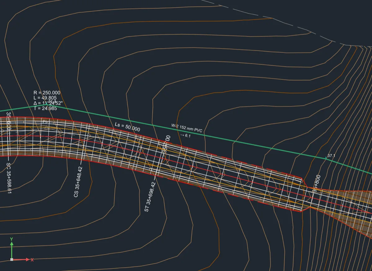
You can exchange networks with EPANET and other tools that read its .inp files.
- Click Pro Analysis ▸ Import EPANET, or type
WNIMPORT, and give the file's path. - Give the Insertion point for the file's coordinates (0,0) and their Scale (1). The file's [COORDINATES] are placed with these.
Terrace makes a pressure network with the file's junctions, reservoirs, tanks (with volume curves), pipes, pumps (curves, power, speed and speed patterns), valves (PRV, PSV, PBV, FCV, TCV and GPV), demands with categories, patterns, curves, simple controls, times and hydraulic options. Pipe lengths come from the file, not from the drawing. Units follow the file's flow units (CFS, GPM, MGD… for US files; LPS, LPM, MLD, CMH, CMD for SI files). Terrace then says what it read and anything it won't analyse:

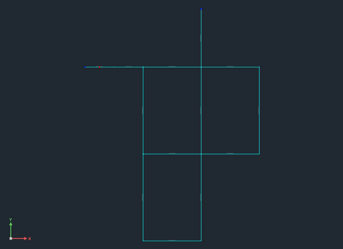
The result labels of a network read from a file grow with the coordinates' scale: with Net1 read at scale 10, they're 10 times the network's own label height, so they keep their size against the pipes.
- Export EPANET (
WNEXPORT): writes a network and its whole setup as an.inpfile you can open in EPANET. WNREPORT(Results CSV… in the Setup tab): writes the results as CSV, every node and every link at every reported time. The node block has Time, Node, Type, Elevation, Demand, Head, Pressure and Check; the link block follows. If the network changed since the run, Terrace says the results are the old ones.
How Terrace checks this, and what it doesn't analyse
Terrace's solver follows EPANET 2.2's method and status rules. It is tested against the EPANET 2.2 toolkit itself, run on EPANET's example networks Net1, Net2 and Net3 and on Terrace's own test networks (every valve type, check valves, three-point, multi-point and constant-power pumps, tanks with and without volume curves, time, clock and level controls, US and SI units, Hazen-Williams and Darcy-Weisbach). At every reported time, every head and pressure agrees within 1 mm, every flow within 0.01 %, and every link's open/closed status matches.
What it doesn't analyse (the import tells you when a file has these):
- Rule-based controls ([RULES]). Simple controls by time, clock time or tank level are analysed.
- Emitters (sprinklers, leakage).
- Water quality (chlorine, age, trace).
- Pressure-driven demand: demands are always met in full.
- Pump energy is an estimate at 75 % wire-to-water efficiency (EPANET's default), not from the file's efficiency curves or energy prices.
Good to know
- Every hydro object and water setup is saved in the
.terracefile and follows its surfaces, alignments and catchments. Rebuild a surface and its ponds, flood maps and reservoirs recompute. - Floods, ponds and reservoirs are measured on the surface you pick. For the water level against the finished road, pick a surface that includes the road, such as a surface pasted from the corridor's Top (see Surfaces).
- At the command line a space works like Enter where Terrace expects an object: to pick a catchment or surface whose name has spaces, click it on the plan. Name prompts (
HYDROREPORT,HYDRODELETE, a lining) take spaces.